#data science #python #geopandas #google earth engine #viirs #qgis #pandas #matplotlib #jupyter
Project Overview
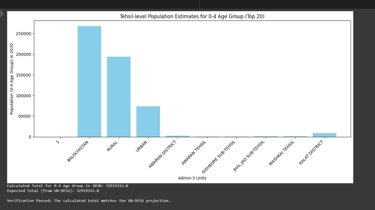
Comprehensive geospatial analysis project examining population distribution patterns and infrastructure development across Pakistan. Integrates 2017 Census data with UN-DESA population projections to analyze children aged 0-4 demographics for 2030. Utilizes Google Earth Engine VIIRS nighttime lights data to assess infrastructure development and urbanization patterns. The project combines multiple administrative boundary levels (tehsil, district, province) with satellite imagery analysis to provide insights into demographic trends and regional development patterns.
Project Overview & Spatial Distribution
Population distribution analysis and spatial visualization of demographic patterns across Pakistan's administrative boundaries.
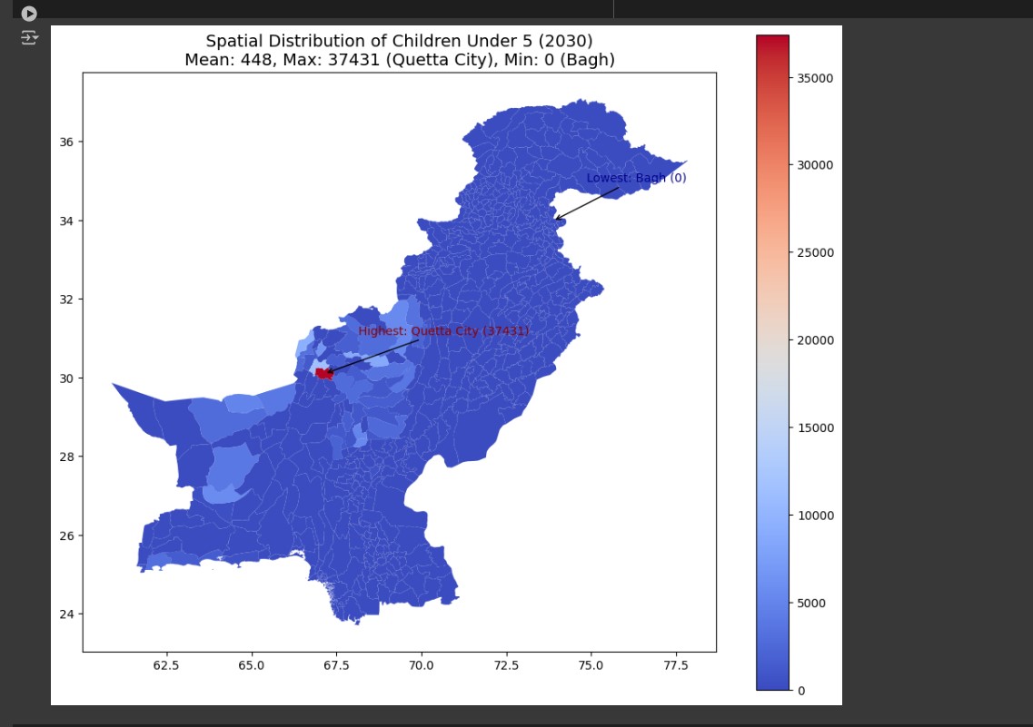
Spatial Population Distribution: Spatial visualization of population patterns showing administrative-level demographic distribution across Pakistan's tehsils.
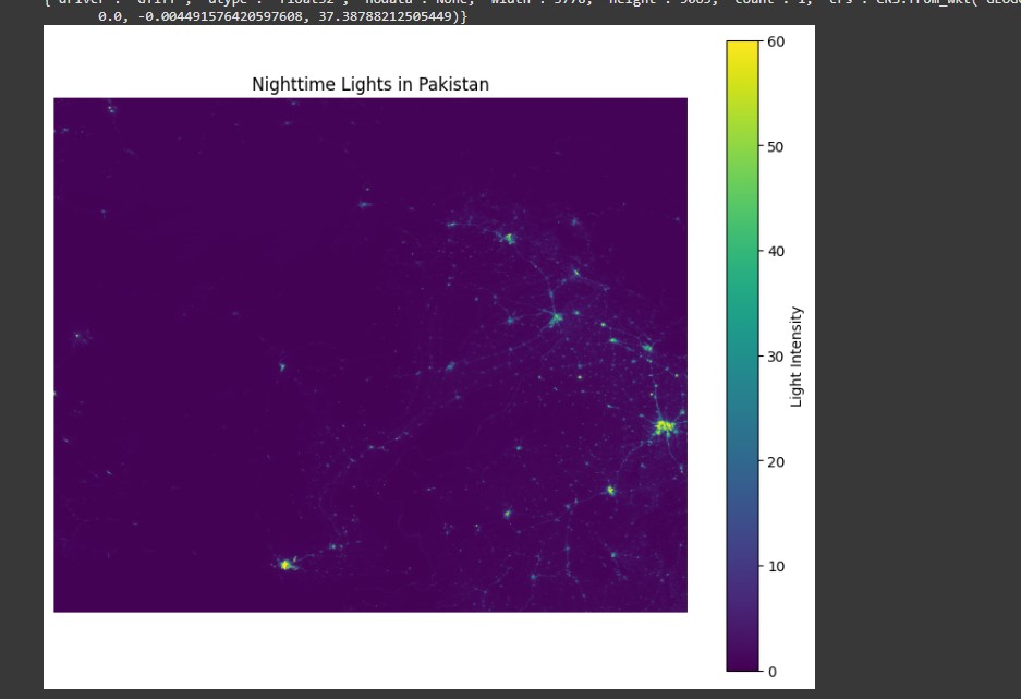
Nighttime Lights Infrastructure Analysis
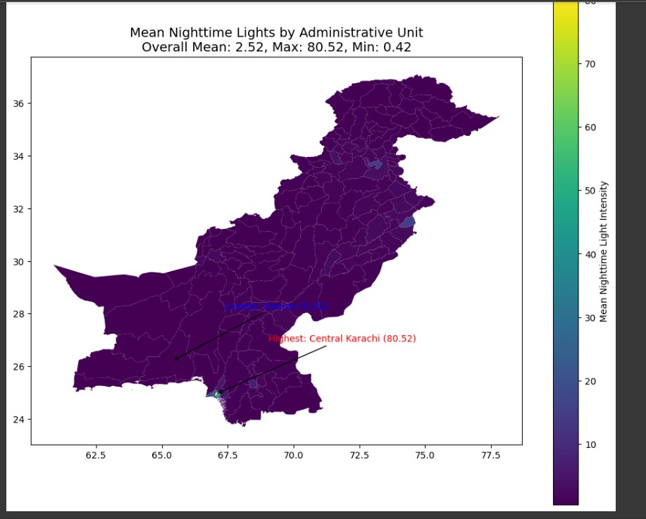
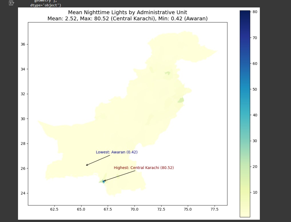
VIIRS satellite data analysis revealing urbanization patterns and infrastructure development across Pakistan.
Light Intensity Heatmap: Heatmap of nighttime light intensity highlighting urbanization levels and development patterns across administrative boundaries.
Project Structure & Data Flow
Organized file structure and data processing pipeline for reproducible spatial analysis.
population_analysis/
├── python/
│   └── Cleaning.ipynb          # Main analysis notebook
├── DataSets/                   # Raw data (external download)
│   ├── pakistan_census_2017/
│   ├── un_desa_projections/
│   └── ocha_boundaries/
├── Cleaned_data/
│   ├── all_tehsil_cleaned.csv
│   ├── all_tehsil_2030.csv
│   └── tehsil_children_0_4_2030.csv
├── Processed_Spatial_Data/
│   ├── final_spatial_distribution.geojson
│   └── Nighttime_Lights_Pakistan.tif
└── Shapefiles/
    ├── Admin_Level_0/          # Country boundaries
    ├── Admin_Level_1/          # Province boundaries
    ├── Admin_Level_2/          # District boundaries
    └── Admin_Level_3/          # Tehsil boundaries
Data Cleaning & Processing Pipeline
Python workflow for processing census data and integrating multiple geospatial datasets.
import pandas as pd
import geopandas as gpd
from rasterstats import zonal_stats
import matplotlib.pyplot as plt

# Data cleaning pipeline for census data
def clean_census_data(file_path, output_path):
    """Clean and standardize Pakistan Census 2017 data"""
    df = pd.read_excel(file_path)

    # Standardize column names and data types
    df.columns = df.columns.str.lower().str.replace(' ', '_')
    df = df.dropna(subset=['tehsil_name', 'total_population'])

    # Calculate children 0-4 demographics
    df['children_0_4'] = df['age_0'] + df['age_1'] + df['age_2'] + df['age_3'] + df['age_4']
    df['children_0_4_percentage'] = (df['children_0_4'] / df['total_population']) * 100

    df.to_csv(output_path, index=False)
    return df

# Project population to 2030 using UN-DESA growth rates
def project_population_2030(census_df, growth_rates):
    """Apply UN-DESA growth rates for 2030 projections"""
    years_diff = 2030 - 2017

    for province in census_df['province'].unique():
        growth_rate = growth_rates.get(province, 0.024)  # default 2.4%
        mask = census_df['province'] == province
        census_df.loc[mask, 'projected_population_2030'] = (
            census_df.loc[mask, 'total_population'] *
            ((1 + growth_rate) ** years_diff)
        )

    return census_df
Geospatial Analysis & Visualization
Integration of demographic data with administrative boundaries and satellite imagery analysis.
import geopandas as gpd
from rasterstats import zonal_stats
import ee

# Initialize Google Earth Engine
ee.Initialize()

def merge_spatial_data(census_df, shapefile_path):
    """Merge census data with administrative boundaries"""
    gdf = gpd.read_file(shapefile_path)

    # Standardize naming for spatial join
    gdf['tehsil_name'] = gdf['ADM3_EN'].str.upper().str.strip()
    census_df['tehsil_name'] = census_df['tehsil_name'].str.upper().str.strip()

    # Spatial merge
    merged_gdf = gdf.merge(census_df, on='tehsil_name', how='left')

    return merged_gdf

def extract_nighttime_lights(boundary_gdf, year=2021):
    """Extract VIIRS nighttime lights using Google Earth Engine"""

    # Load VIIRS DNB collection
    viirs = ee.ImageCollection('NOAA/VIIRS/DNB/ANNUAL_V22') \
              .filterDate(f'{year}-01-01', f'{year}-12-31') \
              .select('avg_rad')

    # Get annual composite
    annual_lights = viirs.median()

    # Export to Google Drive or Cloud Storage
    task = ee.batch.Export.image.toDrive(
        image=annual_lights,
        description='Pakistan_Nighttime_Lights',
        scale=500,
        region=boundary_gdf.total_bounds,
        maxPixels=1e9
    )

    return annual_lights

def calculate_zonal_statistics(boundary_gdf, raster_path):
    """Calculate nighttime lights statistics for each administrative unit"""

    stats = zonal_stats(
        boundary_gdf,
        raster_path,
        stats=['mean', 'sum', 'max', 'count'],
        all_touched=True,
        nodata=-999
    )

    # Add statistics to GeoDataFrame
    for i, stat in enumerate(stats):
        boundary_gdf.loc[i, 'lights_mean'] = stat['mean']
        boundary_gdf.loc[i, 'lights_sum'] = stat['sum']
        boundary_gdf.loc[i, 'lights_max'] = stat['max']

    return boundary_gdf
Data Visualization & Mapping
Creating comprehensive visualizations for demographic and infrastructure analysis.
import matplotlib.pyplot as plt
import seaborn as sns
from mpl_toolkits.axes_grid1 import make_axes_locatable

def create_choropleth_map(gdf, column, title, cmap='YlOrRd'):
    """Create choropleth map for demographic data"""
    fig, ax = plt.subplots(1, 1, figsize=(15, 10))

    # Plot choropleth
    gdf.plot(column=column,
             cmap=cmap,
             linewidth=0.8,
             ax=ax,
             edgecolor='white',
             legend=True,
             legend_kwds={'shrink': 0.8})

    ax.set_title(title, fontsize=16, fontweight='bold')
    ax.set_axis_off()

    # Add province boundaries
    gdf.boundary.plot(ax=ax, linewidth=1, edgecolor='black', alpha=0.5)

    plt.tight_layout()
    return fig

def create_correlation_analysis(merged_gdf):
    """Analyze correlation between population and nighttime lights"""

    # Calculate correlation
    correlation_data = merged_gdf[['projected_population_2030',
                                   'children_0_4',
                                   'lights_mean',
                                   'lights_sum']].corr()

    # Create heatmap
    plt.figure(figsize=(10, 8))
    sns.heatmap(correlation_data,
                annot=True,
                cmap='coolwarm',
                center=0,
                square=True,
                cbar_kws={'shrink': 0.8})

    plt.title('Correlation: Population vs Infrastructure (Nighttime Lights)')
    plt.tight_layout()

    return correlation_data

# Export final results
def export_results(merged_gdf, output_dir):
    """Export processed data in multiple formats"""

    # GeoJSON for web mapping
    merged_gdf.to_file(f"{output_dir}/final_spatial_distribution.geojson",
                       driver='GeoJSON')

    # CSV for statistical analysis
    df_export = merged_gdf.drop('geometry', axis=1)
    df_export.to_csv(f"{output_dir}/spatial_analysis_results.csv", index=False)

    print(f"Results exported to {output_dir}")
    print(f"Total administrative units: {len(merged_gdf)}")
    print(f"Data completeness: {merged_gdf['projected_population_2030'].notna().mean():.1%}")
Data Sources & External Dependencies
External datasets and APIs required for reproducing the analysis.
# External Data Sources
data_sources:
  census:
    source: "Pakistan Bureau of Statistics"
    dataset: "Pakistan 2017 Census"
    url: "https://www.pbs.gov.pk/census-2017"
    format: "Excel/PDF"

  projections:
    source: "UN Department of Economic and Social Affairs"
    dataset: "World Population Prospects 2022"
    url: "https://population.un.org/wpp/downloads"
    format: "CSV"

  boundaries:
    source: "UN Office for the Coordination of Humanitarian Affairs"
    dataset: "Pakistan Administrative Boundaries"
    url: "https://data.humdata.org/dataset/cod-ab-pak"
    format: "Shapefile"

  satellite:
    source: "Google Earth Engine"
    dataset: "NOAA/VIIRS/DNB/ANNUAL_V22"
    description: "VIIRS Day/Night Band Annual Composites"
    access: "Requires Google Earth Engine account"

# Python Dependencies
dependencies:
  core:
    - pandas>=1.3.0
    - geopandas>=0.10.0
    - matplotlib>=3.5.0
    - seaborn>=0.11.0
  geospatial:
    - rasterstats>=0.15.0
    - fiona>=1.8.0
    - shapely>=1.8.0
  google_earth_engine:
    - earthengine-api>=0.1.300
Challenges
Handling large-scale geospatial datasets with varying formats and coordinate systems. Processing and cleaning census data across multiple administrative levels while maintaining spatial accuracy. Integrating satellite nighttime lights data with demographic information required careful spatial joins and statistical analysis. Managing memory constraints when processing high-resolution raster data. Ensuring data consistency across different sources (Census 2017, UN-DESA projections, OCHA shapefiles) with varying temporal and spatial resolutions.
Solutions
Implemented efficient data cleaning pipeline using Python pandas and geopandas for processing census data across all tehsils. Utilized Google Earth Engine API for automated VIIRS nighttime lights data extraction and preprocessing. Developed spatial analysis workflows using rasterstats for zonal statistics computation. Created standardized coordinate reference systems and boundary matching algorithms. Built modular Jupyter notebook structure for reproducible analysis with clear data flow from raw datasets to final visualizations.
Results
Successfully processed and analyzed population data for 2030 projections covering all administrative units in Pakistan. Generated comprehensive spatial distribution maps showing children under 5 demographics with administrative boundary overlays. Produced nighttime lights intensity analysis revealing urbanization patterns and infrastructure development levels. Created exportable GeoJSON files for web mapping applications and TIFF rasters for GIS analysis. Established reproducible workflow that can be adapted for other countries or demographic groups. The analysis provides valuable insights for policy makers regarding child welfare resource allocation and infrastructure development planning.
Technologies Used
PythonGeoPandasGoogle Earth EngineVIIRSQGISPandasMatplotlibJupyter